10 Characterising Random Fields
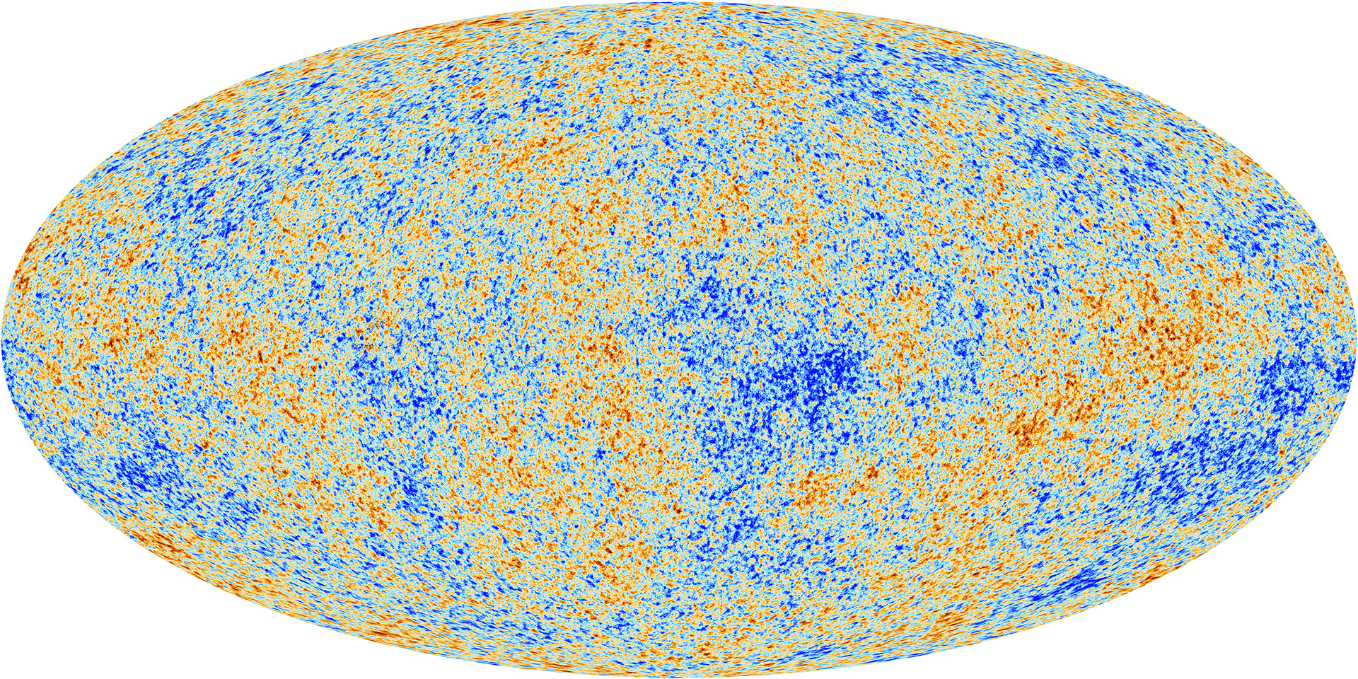
The real universe is far from homogeneous and isotropic except on the largest scales. Figure 12 (left panel) shows slices through the 3D distribution of galaxy positions from the 2dF galaxy redshift survey out to a comoving distance of . The distribution of galaxies is clearly not random; instead they are arranged into a delicate cosmic web with galaxies strung out along dense filaments and clustering at their intersections, leaving huge empty voids. However, if we smooth the picture on large scales () it starts to look much more homogeneous. Furthermore, we know from the CMB that the universe was smooth to around 1 part in at the time of recombination; see right panel of Fig. 12. The aim of the rest of the course is to study the growth of large-scale structure in an expanding universe through gravitational instability acting on small initial perturbations. We will then learn how these initial perturbations were likely produced by quantum effects during cosmological inflation.
 |
In this Chapter, we will explore the basic statistical properties enforced on such fields by assuming the physics that generates the initial fluctuations, and subsequently processes them, respects the symmetries of the background cosmology, i.e. isotropy and homogeneity. It seems inconsistent at first sight to talk about inhomogeneities/anisotropies being generated by a mechanism that is itself homogeneous/isotropic! But there is a key distinction: it is homogeneous and isotropic on average over all possible universes but not for a specific universe such as our own.
Throughout, we denote expectation values with angle brackets, For some quantity , we imagine measuring it in different universes and getting different results , , , . Then the expectation value is defined by
| (265) |
To be clear, one will never be able to actually measure (irrespective of what represents) because it requires access to an infinity of different universes. But it is still a useful theoretical construction as we shall see.
10.1 The two-point correlation function in 3D Euclidean space
Consider a random field – i.e. at each point is some random number – with zero mean, . Correlators of fields are expectation values of products of fields at different spatial points (and, possibly, different times). They are important because typically they can be calculated theoretically, and can be estimated observationally; they are the essential link between observation and theory (see Section 6 below).
The two point correlator of the field is defined by
| (266) |
where again is the field evaluated at in the th notional universe.
We can now explore some general properties of . Statistical homogeneity means that the statistical properties of the translated field are the same as the original field. For the two-point correlation, this implies
| (267) |
so the two-point correlator only depends on the separation of the two points. As a shorthand, we therefore can write , discarding the trailing .
Statistical isotropy means that the statistical properties of the rotated field are the same as the original field. For the two-point correlator, we must have
| (268) |
Combining statistical homogeneity and isotropy gives
| (269) |
so the two-point correlator depends only on the distance between the two points. We therefore write , both discarding the trailing (as before) but also being clear that is a function only of the scalar separation of and , not of orientation. You can verify that this holds even if correlating different fields (or the same field at different times).
10.2 Random fields in Fourier space
We can repeat these arguments to constrain the form of the correlators in Fourier space, which we will use in preference to the real-space results above. We adopt the symmetric Fourier convention, so that
| (270) |
Note that we don’t use a different notation for the function ; whether we are talking about the function evaluated in the Fourier or real-space domains is normally very clear from the context. While some textbooks use a different symbol such as , this becomes extremely fussy for complicated expressions and so we will not bother.
For real fields it follows immediately from the definitions above that . Also recall that spatial derivatives turn into factors of in the Fourier transform, e.g. the fourier transform of is
| (271) |
Similarly the Fourier transform of is . These properties will be important to us when we develop perturbation theory in Sections 11 and 13, allowing us to replace differential equations in real space with algebraic ones in Fourier space .
For now, we need to focus on a different property; namely, under translations, the Fourier transform acquires a phase factor:
| (272) |
Let’s consider the two-point correlator in Fourier space. We could write this but actually we instead by convention consider . (The two options contain equivalent information, but the second turns out to lead to simpler mathematical expressions.) Invariance of the two-point correlator in Fourier space under translations implies
| (273) |
for some function , where indicates the Dirac delta function which is zero when . The upshot is that different Fourier modes are necessarily uncorrelated due to statistical homogeneity. Under rotations,
where . Now, for any rotation matrix , we have . So, , and
| (275) | ||||
| (276) |
So demanding invariance of the two-point correlator under rotations implies
| (277) |
(To get this result you need to use property of the Dirac delta function .) Equation (277) can only hold if where . We can therefore define the power spectrum, , of a homogeneous and isotropic field, , by
| (278) |
The normalisation factor in the definition of the power spectrum is conventional and has the virtue of making dimensionless if is.
10.3 Relationship between the correlation function and the power spectrum
The correlation function and the power spectrum carry the same physical information, just in a different form. To get the detailed relationship requires a bit of algebra. First, we write down the correlation function and substitute the inverse Fourier transforms (270):
| (279) |
where we made use of the fact that is real to replace it with its own complex conjugate. (This is just a minor trick to simplify the algebra a little.) The term can be replaced by the power spectrum using equation (278), after which the integral can be performed. We also write where is a unit vector containing the direction information in . This gets us to the following expression:
| (280) |
We can evaluate the integral over by setting , the integral then reduces to
| (281) |
It follows that the sought-after relationship between and is:
| (282) |
Note that this only depends on as required by the translational and rotational invariance that we discussed earlier.
10.4 Gaussianity
Inflation predicts fluctuations that are very nearly Gaussian and this property is preserved by linear evolution. The cosmic microwave background probes fluctuations mostly in this linear regime (see right panel of Fig. 12).
When we say that the field is Gaussian, we mean first that the probability of finding a particular value at a given location can be written as a Gaussian:
| (283) |
Since, from the definitions above, we must have , the value of is just given by . By saying the field is Gaussian we also mean that the probability density for the field taking on specified values at multiple points – say , , , – is given by a multivariate Guassian, with covariance given by:
| (284) |
i.e. fully specified just by the correlation function. So the real point of a Gaussian field is that these 2-point correlations capture all the information. There is no further information in higher order correlators.
Why should the fluctuations emerging from inflation be nearly Gaussian? If you have studied quantum field theory (QFT), the answer is pretty clear: when we calculate the 2-point correlator of a quantum field , the result is given to us by the QFT propagator. But when we calculate higher-order correlations such as , we turn to interacting field theory where there are not just propagators but also interaction vertices; these carry at least one factor of the interaction strength which is typically small.
Non-linear structure formation at late times destroys Gaussianity and gives the filamentary cosmic web (see left panel of Fig. 12). So the late time universe is certainly non-Gaussian. But searching for primordial non-Gaussianity to probe departures from simple inflation is a hot topic; no convincing evidence for primordial non-Gaussianity has yet been found.
10.5 Random fields on the sphere
Physical fields (in a flat universe) can be represented in Fourier or real space as described above. We’ve seen that an ability to work in Fourier space is essential because it allows us to encode notions like homogeneity and isotropy of the field statistics in a succinct way – equation (278).
However observations at their root consist of a field associated with position on the sky – we can think of observations as measured fields on the surface of a sphere. For that reason we need to be able to express fields on the surface of a sphere and manipulate them with the same sophistication as we can for fields in flat space.
Spherical harmonics are basis functions on the sphere that are the closest possible equivalent to Fourier modes. Functions of position on the sphere can be expanded as
| (285) |
In this expression and others involving spherical harmonics we normally don’t use the summation convention, i.e. repeated indices do not implicitly mean a sum. We instead write sums explicitly where required, as in Eq. (285). The are familiar2323 23 Just to ward off potential confusion – there are various phase conventions for the ; here we adopt so that for a real field. from quantum mechanics as the position-space representation of the eigenstates of and :
| (286) |
with an integer and an integer with . This implies a typical wavelength of fluctuations for a given : because , we are talking about fluctuations with an angular scale of
| (287) |
Note the close analogy with Fourier modes in a flat space where and . In the Fourier case, the scale of fluctuations is . So acts a bit like the wavenumber whereas is a bit like (i.e. contains information about directionality).
Just like the Fourier modes, the spherical harmonics have a lot of special properties that help us manipulate them. They are orthonormal over the sphere,
| (288) |
so that the spherical multipole coefficients of are
| (289) |
In turn, this implies a completeness relationship
| (290) |
where is the Dirac delta function on the sphere.
There is a generalisation of equation (290) which sums only over the s, not the s. It is known as the spherical harmonic addition theorem and states that
| (291) |
where is the ’th Legendre polynomial. Many different proofs of this statement are available e.g. in quantum mechanics text books. They’re a bit tedious so here we’ll just take the result on trust (we’ll only need it once anyway).
What is the implication of statistical isotropy for the correlators of ? We first need to know that, under a rotation, for some rotation coefficients ; any given rotation of a general function can therefore be effected by transforming its spherical harmonic coefficients . There are a few helpful properties of the :
-
•
They do not mix different s (this is already built into the notation). If you’re curious to see why, you can show it from the commutation of with the individual rotation generators.
-
•
It’s relatively straight-forward to show that – this can be derived from the orthonormalisation of the s themselves.
-
•
There is an extension of the previous statement that is even more powerful: namely, the ’s are orthonormalized such that . Demonstrating this requires application of the completeness relation (290) and is recommended for enthusiasts only.
-
•
For a rotation of angle around the z axis, . This follows directly from equation (286).
 Exercise 10B
Show that the above conditions are not just sufficient but also necessary
for isotropy.
Exercise 10B
Show that the above conditions are not just sufficient but also necessary
for isotropy.
10.6 Estimating the properties of random fields
Random fields are defined by their ensemble average properties. If some element of randomness is involved in physics (e.g. because of quantum mechanics) we would ideally want to measure ensemble average outcomes rather than an individual outcome.
However in cosmology, this isn’t an option – we have just one universe and we’re stuck with it. Yet, if one makes sufficiently strong assumptions (normally homogeneity and isotropy), it’s still possible to make inferences about the random process. In effect, one splits up the data into lots of chunks and regards them as independent “trials” of the random process. This introduces inherent limits to what can be achieved – especially when we’re talking about the very largest scales of the universe. If and when we find something that seems strange or doesn’t fit the model, we must bear in mind that we might just be looking at an “unlucky” draw from the random process.
Later in the course we will especially look at the cosmic microwave background, which is an example of a random field on a notional sphere (the “surface of last scattering”). We want to be able to measure , but in practice we can’t because – we’re unable to take the required ensemble average from within our own universe.
Instead we construct an “estimator for ” which does what the name suggests: it estimates from a single observation. Such estimators are normally written ; the simplest (and, in ideal circumstances, the best) example of which is:
| (294) |
☞ Exercise 10C
Show that the estimator has expectation and variance:
| (295) |
You may want to use Wick’s theorem, which states that for zero-mean Gaussian random numbers , , and , .
The exercise above shows that on average, will be close to , especially as becomes large (this corresponds to small scales where there are lots of independent modes each sampling ). But for small – the largest accessible angular scales – the standard deviation becomes comparable to itself. This inherent limitation in our ability to estimate (or other statistical properties of fields we observe) is known as “cosmic variance”.
10.7 Summary
-
•
Many of the predictions made by modern cosmological theories are statistical in nature;
-
•
Quantum fields have near-Gaussian random fluctuations which, in the inflationary picture, seed structure in our Universe;
-
•
Gaussian fluctuations can be characterised by two-point correlations alone;
-
•
Statistical homogeneity and isotropy put stringent limitations on the form that two-point correlations can take;
-
•
The predictions then take the form of a power spectrum , measuring fluctuations on comoving scales – or, equivalently, a correlation function ;
-
•
When measured on a sphere, the power spectrum is discretised into ’s measuring fluctuations on angular scales
-
•
Power spectra can be calculated from theories but cannot be measured directly from observations because they involve an average over an infinite series of universes…
-
•
…however we can estimate power spectra observationally by averaging over a number of observed modes. The theory/observation comparison will then have an irreducible level of uncertainty known as “cosmic variance”. This is most problematic when probing large scales due to the small number of accessible large-scale modes.